최적화의 솔루션 공간 컨투어링

등고선 플로팅은 최적화 문제의 솔루션 공간을 설명할 때 특히 유용합니다. axes.Axes.contour목적 함수의 지형을 나타내는 데 사용할 수 있을 뿐만 아니라 제약 함수의 경계 곡선을 생성하는 데 사용할 수 있습니다. TickedStroke구속 조건 경계의 유효면과 무효면을 구분하기 위해 구속선을 그릴 수 있습니다 .

axes.Axes.contour윤곽선 왼쪽에 더 큰 값을 가진 곡선을 생성합니다. 각도 매개변수는 왼쪽으로 값이 증가하면서 0점 앞으로 측정됩니다. 따라서 TickedStroke일반적인 최적화 문제에서 제약 조건을 설명하기 위해 를 사용할 때 각도는 0도에서 180도 사이로 설정해야 합니다.

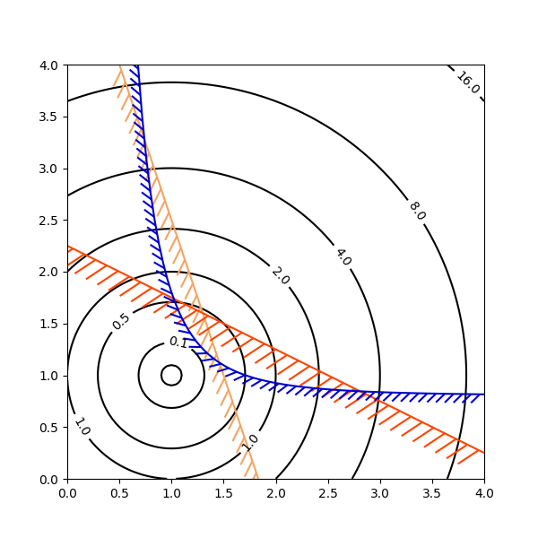
import numpy as np
import matplotlib.pyplot as plt
from matplotlib import patheffects

fig, ax = plt.subplots(figsize=(6, 6))

nx = 101
ny = 105

# Set up survey vectors
xvec = np.linspace(0.001, 4.0, nx)
yvec = np.linspace(0.001, 4.0, ny)

# Set up survey matrices.  Design disk loading and gear ratio.
x1, x2 = np.meshgrid(xvec, yvec)

# Evaluate some stuff to plot
obj = x1**2 + x2**2 - 2*x1 - 2*x2 + 2
g1 = -(3*x1 + x2 - 5.5)
g2 = -(x1 + 2*x2 - 4.5)
g3 = 0.8 + x1**-3 - x2

cntr = ax.contour(x1, x2, obj, [0.01, 0.1, 0.5, 1, 2, 4, 8, 16],
                  colors='black')
ax.clabel(cntr, fmt="%2.1f", use_clabeltext=True)

cg1 = ax.contour(x1, x2, g1, [0], colors='sandybrown')
plt.setp(cg1.collections,
         path_effects=[patheffects.withTickedStroke(angle=135)])

cg2 = ax.contour(x1, x2, g2, [0], colors='orangered')
plt.setp(cg2.collections,
         path_effects=[patheffects.withTickedStroke(angle=60, length=2)])

cg3 = ax.contour(x1, x2, g3, [0], colors='mediumblue')
plt.setp(cg3.collections,
         path_effects=[patheffects.withTickedStroke(spacing=7)])

ax.set_xlim(0, 4)
ax.set_ylim(0, 4)

plt.show()