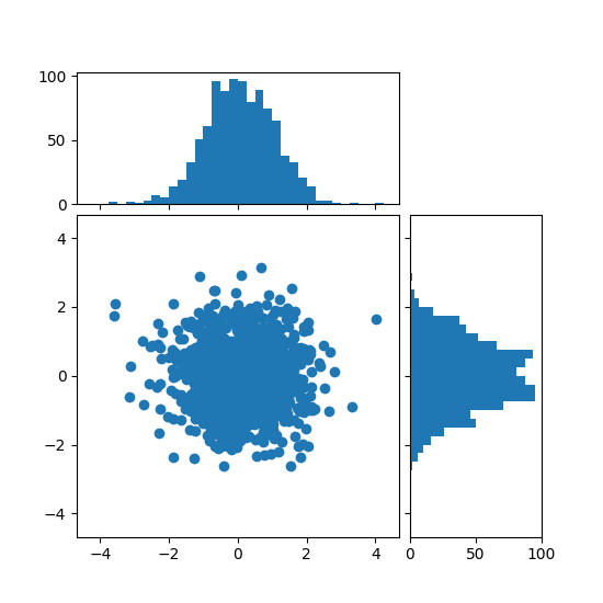
분산형 히스토그램(찾을 수 있는 축) #

플롯의 측면에 히스토그램으로 산점도의 주변 분포를 표시합니다.

주축과 주변축의 좋은 정렬을 위해 축 위치는 Divider를 통해 생성되는 에 의해 정의됩니다 make_axes_locatable. API를 사용 하면 Divider주요 기능인 축 크기와 패드를 인치 단위로 설정할 수 있습니다.

기본 그림을 기준으로 축 크기와 패드를 설정하려면 히스토그램 예제 가 있는 산점도 를 참조하십시오.

import numpy as np
import matplotlib.pyplot as plt
from mpl_toolkits.axes_grid1 import make_axes_locatable

# Fixing random state for reproducibility
np.random.seed(19680801)

# the random data
x = np.random.randn(1000)
y = np.random.randn(1000)


fig, ax = plt.subplots(figsize=(5.5, 5.5))

# the scatter plot:
ax.scatter(x, y)

# Set aspect of the main axes.
ax.set_aspect(1.)

# create new axes on the right and on the top of the current axes
divider = make_axes_locatable(ax)
# below height and pad are in inches
ax_histx = divider.append_axes("top", 1.2, pad=0.1, sharex=ax)
ax_histy = divider.append_axes("right", 1.2, pad=0.1, sharey=ax)

# make some labels invisible
ax_histx.xaxis.set_tick_params(labelbottom=False)
ax_histy.yaxis.set_tick_params(labelleft=False)

# now determine nice limits by hand:
binwidth = 0.25
xymax = max(np.max(np.abs(x)), np.max(np.abs(y)))
lim = (int(xymax/binwidth) + 1)*binwidth

bins = np.arange(-lim, lim + binwidth, binwidth)
ax_histx.hist(x, bins=bins)
ax_histy.hist(y, bins=bins, orientation='horizontal')

# the xaxis of ax_histx and yaxis of ax_histy are shared with ax,
# thus there is no need to manually adjust the xlim and ylim of these
# axis.

ax_histx.set_yticks([0, 50, 100])
ax_histy.set_xticks([0, 50, 100])

plt.show()

참조

다음 함수, 메서드, 클래스 및 모듈의 사용이 이 예제에 표시됩니다.

Sphinx-Gallery에서 생성한 갤러리