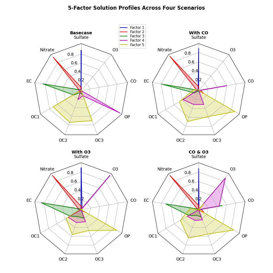
레이더 차트(거미 또는 스타 차트라고도 함) #

이 예에서는 거미 또는 별 차트 [ 1 ] 라고도 하는 방사형 차트를 만듭니다 .

이 예제에서는 '원' 또는 '다각형' 프레임을 허용하지만 다각형 프레임에는 적절한 격자선이 없습니다(선은 다각형이 아닌 원임). matplotlib.axis의 GRIDLINE_INTERPOLATION_STEPS를 원하는 정점 수로 설정하여 다각형 그리드를 얻을 수 있지만 다각형의 방향이 방사형 축과 정렬되지 않습니다.

import numpy as np

import matplotlib.pyplot as plt
from matplotlib.patches import Circle, RegularPolygon
from matplotlib.path import Path
from matplotlib.projections.polar import PolarAxes
from matplotlib.projections import register_projection
from matplotlib.spines import Spine
from matplotlib.transforms import Affine2D


def radar_factory(num_vars, frame='circle'):
    """
    Create a radar chart with `num_vars` axes.

    This function creates a RadarAxes projection and registers it.

    Parameters
    ----------
    num_vars : int
        Number of variables for radar chart.
    frame : {'circle', 'polygon'}
        Shape of frame surrounding axes.

    """
    # calculate evenly-spaced axis angles
    theta = np.linspace(0, 2*np.pi, num_vars, endpoint=False)

    class RadarTransform(PolarAxes.PolarTransform):

        def transform_path_non_affine(self, path):
            # Paths with non-unit interpolation steps correspond to gridlines,
            # in which case we force interpolation (to defeat PolarTransform's
            # autoconversion to circular arcs).
            if path._interpolation_steps > 1:
                path = path.interpolated(num_vars)
            return Path(self.transform(path.vertices), path.codes)

    class RadarAxes(PolarAxes):

        name = 'radar'
        PolarTransform = RadarTransform

        def __init__(self, *args, **kwargs):
            super().__init__(*args, **kwargs)
            # rotate plot such that the first axis is at the top
            self.set_theta_zero_location('N')

        def fill(self, *args, closed=True, **kwargs):
            """Override fill so that line is closed by default"""
            return super().fill(closed=closed, *args, **kwargs)

        def plot(self, *args, **kwargs):
            """Override plot so that line is closed by default"""
            lines = super().plot(*args, **kwargs)
            for line in lines:
                self._close_line(line)

        def _close_line(self, line):
            x, y = line.get_data()
            # FIXME: markers at x[0], y[0] get doubled-up
            if x[0] != x[-1]:
                x = np.append(x, x[0])
                y = np.append(y, y[0])
                line.set_data(x, y)

        def set_varlabels(self, labels):
            self.set_thetagrids(np.degrees(theta), labels)

        def _gen_axes_patch(self):
            # The Axes patch must be centered at (0.5, 0.5) and of radius 0.5
            # in axes coordinates.
            if frame == 'circle':
                return Circle((0.5, 0.5), 0.5)
            elif frame == 'polygon':
                return RegularPolygon((0.5, 0.5), num_vars,
                                      radius=.5, edgecolor="k")
            else:
                raise ValueError("Unknown value for 'frame': %s" % frame)

        def _gen_axes_spines(self):
            if frame == 'circle':
                return super()._gen_axes_spines()
            elif frame == 'polygon':
                # spine_type must be 'left'/'right'/'top'/'bottom'/'circle'.
                spine = Spine(axes=self,
                              spine_type='circle',
                              path=Path.unit_regular_polygon(num_vars))
                # unit_regular_polygon gives a polygon of radius 1 centered at
                # (0, 0) but we want a polygon of radius 0.5 centered at (0.5,
                # 0.5) in axes coordinates.
                spine.set_transform(Affine2D().scale(.5).translate(.5, .5)
                                    + self.transAxes)
                return {'polar': spine}
            else:
                raise ValueError("Unknown value for 'frame': %s" % frame)

    register_projection(RadarAxes)
    return theta


def example_data():
    # The following data is from the Denver Aerosol Sources and Health study.
    # See doi:10.1016/j.atmosenv.2008.12.017
    #
    # The data are pollution source profile estimates for five modeled
    # pollution sources (e.g., cars, wood-burning, etc) that emit 7-9 chemical
    # species. The radar charts are experimented with here to see if we can
    # nicely visualize how the modeled source profiles change across four
    # scenarios:
    #  1) No gas-phase species present, just seven particulate counts on
    #     Sulfate
    #     Nitrate
    #     Elemental Carbon (EC)
    #     Organic Carbon fraction 1 (OC)
    #     Organic Carbon fraction 2 (OC2)
    #     Organic Carbon fraction 3 (OC3)
    #     Pyrolyzed Organic Carbon (OP)
    #  2)Inclusion of gas-phase specie carbon monoxide (CO)
    #  3)Inclusion of gas-phase specie ozone (O3).
    #  4)Inclusion of both gas-phase species is present...
    data = [
        ['Sulfate', 'Nitrate', 'EC', 'OC1', 'OC2', 'OC3', 'OP', 'CO', 'O3'],
        ('Basecase', [
            [0.88, 0.01, 0.03, 0.03, 0.00, 0.06, 0.01, 0.00, 0.00],
            [0.07, 0.95, 0.04, 0.05, 0.00, 0.02, 0.01, 0.00, 0.00],
            [0.01, 0.02, 0.85, 0.19, 0.05, 0.10, 0.00, 0.00, 0.00],
            [0.02, 0.01, 0.07, 0.01, 0.21, 0.12, 0.98, 0.00, 0.00],
            [0.01, 0.01, 0.02, 0.71, 0.74, 0.70, 0.00, 0.00, 0.00]]),
        ('With CO', [
            [0.88, 0.02, 0.02, 0.02, 0.00, 0.05, 0.00, 0.05, 0.00],
            [0.08, 0.94, 0.04, 0.02, 0.00, 0.01, 0.12, 0.04, 0.00],
            [0.01, 0.01, 0.79, 0.10, 0.00, 0.05, 0.00, 0.31, 0.00],
            [0.00, 0.02, 0.03, 0.38, 0.31, 0.31, 0.00, 0.59, 0.00],
            [0.02, 0.02, 0.11, 0.47, 0.69, 0.58, 0.88, 0.00, 0.00]]),
        ('With O3', [
            [0.89, 0.01, 0.07, 0.00, 0.00, 0.05, 0.00, 0.00, 0.03],
            [0.07, 0.95, 0.05, 0.04, 0.00, 0.02, 0.12, 0.00, 0.00],
            [0.01, 0.02, 0.86, 0.27, 0.16, 0.19, 0.00, 0.00, 0.00],
            [0.01, 0.03, 0.00, 0.32, 0.29, 0.27, 0.00, 0.00, 0.95],
            [0.02, 0.00, 0.03, 0.37, 0.56, 0.47, 0.87, 0.00, 0.00]]),
        ('CO & O3', [
            [0.87, 0.01, 0.08, 0.00, 0.00, 0.04, 0.00, 0.00, 0.01],
            [0.09, 0.95, 0.02, 0.03, 0.00, 0.01, 0.13, 0.06, 0.00],
            [0.01, 0.02, 0.71, 0.24, 0.13, 0.16, 0.00, 0.50, 0.00],
            [0.01, 0.03, 0.00, 0.28, 0.24, 0.23, 0.00, 0.44, 0.88],
            [0.02, 0.00, 0.18, 0.45, 0.64, 0.55, 0.86, 0.00, 0.16]])
    ]
    return data


if __name__ == '__main__':
    N = 9
    theta = radar_factory(N, frame='polygon')

    data = example_data()
    spoke_labels = data.pop(0)

    fig, axs = plt.subplots(figsize=(9, 9), nrows=2, ncols=2,
                            subplot_kw=dict(projection='radar'))
    fig.subplots_adjust(wspace=0.25, hspace=0.20, top=0.85, bottom=0.05)

    colors = ['b', 'r', 'g', 'm', 'y']
    # Plot the four cases from the example data on separate axes
    for ax, (title, case_data) in zip(axs.flat, data):
        ax.set_rgrids([0.2, 0.4, 0.6, 0.8])
        ax.set_title(title, weight='bold', size='medium', position=(0.5, 1.1),
                     horizontalalignment='center', verticalalignment='center')
        for d, color in zip(case_data, colors):
            ax.plot(theta, d, color=color)
            ax.fill(theta, d, facecolor=color, alpha=0.25, label='_nolegend_')
        ax.set_varlabels(spoke_labels)

    # add legend relative to top-left plot
    labels = ('Factor 1', 'Factor 2', 'Factor 3', 'Factor 4', 'Factor 5')
    legend = axs[0, 0].legend(labels, loc=(0.9, .95),
                              labelspacing=0.1, fontsize='small')

    fig.text(0.5, 0.965, '5-Factor Solution Profiles Across Four Scenarios',
             horizontalalignment='center', color='black', weight='bold',
             size='large')

    plt.show()

참조

다음 함수, 메서드, 클래스 및 모듈의 사용이 이 예제에 표시됩니다.

스크립트의 총 실행 시간: (0분 1.611초)

Sphinx-Gallery에서 생성한 갤러리