pcolormesh #

axes.Axes.pcolormesh2D 이미지 스타일 플롯을 생성할 수 있습니다. 유사한 것보다 빠릅니다 pcolor.

import matplotlib.pyplot as plt
from matplotlib.colors import BoundaryNorm
from matplotlib.ticker import MaxNLocator
import numpy as np

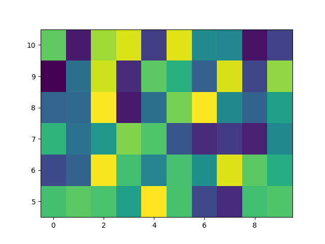
기본 pcolormesh #

우리는 일반적으로 사변형의 가장자리와 사변형의 값을 정의하여 pcolormesh를 지정합니다. 여기서 x 와 y 는 각각 해당 차원에서 Z보다 하나의 추가 요소를 가집니다.

np.random.seed(19680801)
Z = np.random.rand(6, 10)
x = np.arange(-0.5, 10, 1)  # len = 11
y = np.arange(4.5, 11, 1)  # len = 7

fig, ax = plt.subplots()
ax.pcolormesh(x, y, Z)

<matplotlib.collections.QuadMesh object at 0x7f2d00aaeef0>

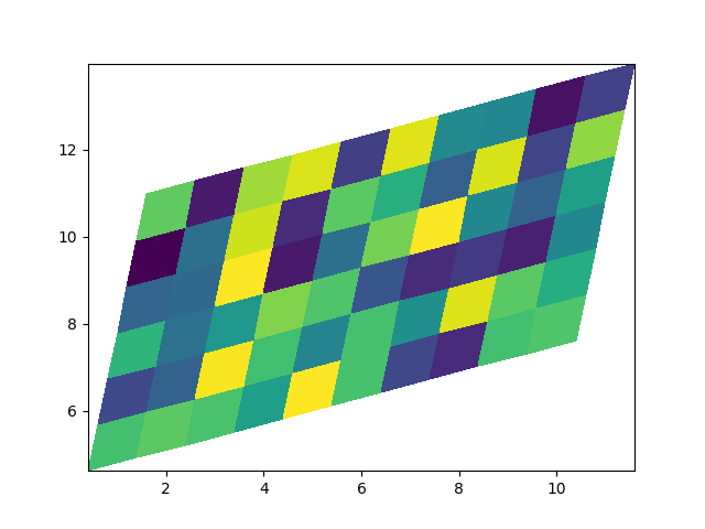
비직선 pcolormesh #

X 와 Y 에 대한 행렬을 지정할 수도 있고 비직선 사변형을 가질 수도 있습니다.

x = np.arange(-0.5, 10, 1)  # len = 11
y = np.arange(4.5, 11, 1)  # len = 7
X, Y = np.meshgrid(x, y)
X = X + 0.2 * Y  # tilt the coordinates.
Y = Y + 0.3 * X

fig, ax = plt.subplots()
ax.pcolormesh(X, Y, Z)

<matplotlib.collections.QuadMesh object at 0x7f2d00c610f0>

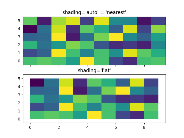
중심 좌표 #

종종 사용자는 Z 와 같은 크기의 X 와 Y 를 에 전달하려고 합니다 . 가 전달된 경우에도 허용됩니다 (기본값은 (기본값: )으로 설정됨). Pre Matplotlib 3.3에서는 Z 의 마지막 열과 행을 삭제합니다 . 이전 버전과의 호환성을 위해 여전히 허용되지만 DeprecationWarning이 발생합니다. 이것이 정말로 원하는 것이라면 Z의 마지막 행과 열을 수동으로 삭제하십시오.axes.Axes.pcolormeshshading='auto'rcParams["pcolor.shading"]'auto'shading='flat'

x = np.arange(10)  # len = 10
y = np.arange(6)  # len = 6
X, Y = np.meshgrid(x, y)

fig, axs = plt.subplots(2, 1, sharex=True, sharey=True)
axs[0].pcolormesh(X, Y, Z, vmin=np.min(Z), vmax=np.max(Z), shading='auto')
axs[0].set_title("shading='auto' = 'nearest'")
axs[1].pcolormesh(X, Y, Z[:-1, :-1], vmin=np.min(Z), vmax=np.max(Z),
                  shading='flat')
axs[1].set_title("shading='flat'")

Text(0.5, 1.0, "shading='flat'")

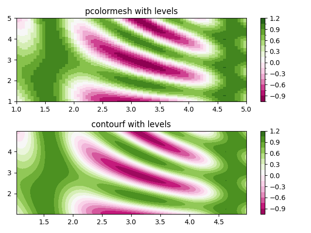
규범을 사용하여 레벨 만들기 #

Normalization 및 Colormap 인스턴스를 결합하여 에서 "레벨"을 그리는 axes.Axes.pcolor방법 과 contour/contourf에 대한 레벨 키워드 인수와 유사한 방식으로 플롯을 입력하는 axes.Axes.pcolormesh 방법 을 보여줍니다.axes.Axes.imshow

# make these smaller to increase the resolution
dx, dy = 0.05, 0.05

# generate 2 2d grids for the x & y bounds
y, x = np.mgrid[slice(1, 5 + dy, dy),
                slice(1, 5 + dx, dx)]

z = np.sin(x)**10 + np.cos(10 + y*x) * np.cos(x)

# x and y are bounds, so z should be the value *inside* those bounds.
# Therefore, remove the last value from the z array.
z = z[:-1, :-1]
levels = MaxNLocator(nbins=15).tick_values(z.min(), z.max())


# pick the desired colormap, sensible levels, and define a normalization
# instance which takes data values and translates those into levels.
cmap = plt.colormaps['PiYG']
norm = BoundaryNorm(levels, ncolors=cmap.N, clip=True)

fig, (ax0, ax1) = plt.subplots(nrows=2)

im = ax0.pcolormesh(x, y, z, cmap=cmap, norm=norm)
fig.colorbar(im, ax=ax0)
ax0.set_title('pcolormesh with levels')


# contours are *point* based plots, so convert our bound into point
# centers
cf = ax1.contourf(x[:-1, :-1] + dx/2.,
                  y[:-1, :-1] + dy/2., z, levels=levels,
                  cmap=cmap)
fig.colorbar(cf, ax=ax1)
ax1.set_title('contourf with levels')

# adjust spacing between subplots so `ax1` title and `ax0` tick labels
# don't overlap
fig.tight_layout()

plt.show()

참조

다음 함수, 메서드, 클래스 및 모듈의 사용이 이 예제에 표시됩니다.

스크립트의 총 실행 시간: (0분 1.467초)

Sphinx-Gallery에서 생성한 갤러리