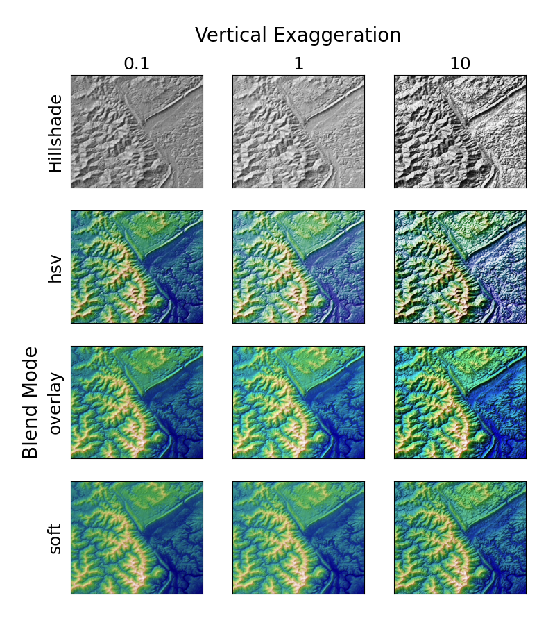
지형 음영기복

"hillshaded" 플롯에서 다양한 블렌드 모드 및 수직 과장의 시각적 효과를 보여줍니다.

"오버레이" 및 "부드러운" 블렌드 모드는 이 예제와 같은 복잡한 표면에 잘 작동하는 반면 기본 "hsv" 블렌드 모드는 많은 수학 함수와 같은 매끄러운 표면에 가장 적합합니다.

대부분의 경우 음영기복은 순전히 시각적인 목적으로 사용되며 dx / dy 는 무시해도 됩니다. 이 경우 시행 착오를 통해 vert_exag (수직 과장)를 조정하여 원하는 시각적 효과를 얻을 수 있습니다. 그러나 이 예는 dx 및 dy 키워드 인수를 사용하여 vert_exag 매개변수가 진정한 수직 과장인지 확인하는 방법을 보여줍니다.

import numpy as np
import matplotlib.pyplot as plt
from matplotlib.cbook import get_sample_data
from matplotlib.colors import LightSource


dem = get_sample_data('jacksboro_fault_dem.npz', np_load=True)
z = dem['elevation']
# -- Optional dx and dy for accurate vertical exaggeration --------------------
# If you need topographically accurate vertical exaggeration, or you don't want
# to guess at what *vert_exag* should be, you'll need to specify the cellsize
# of the grid (i.e. the *dx* and *dy* parameters).  Otherwise, any *vert_exag*
# value you specify will be relative to the grid spacing of your input data
# (in other words, *dx* and *dy* default to 1.0, and *vert_exag* is calculated
# relative to those parameters).  Similarly, *dx* and *dy* are assumed to be in
# the same units as your input z-values.  Therefore, we'll need to convert the
# given dx and dy from decimal degrees to meters.
dx, dy = dem['dx'], dem['dy']
dy = 111200 * dy
dx = 111200 * dx * np.cos(np.radians(dem['ymin']))
# -----------------------------------------------------------------------------

# Shade from the northwest, with the sun 45 degrees from horizontal
ls = LightSource(azdeg=315, altdeg=45)
cmap = plt.cm.gist_earth

fig, axs = plt.subplots(nrows=4, ncols=3, figsize=(8, 9))
plt.setp(axs.flat, xticks=[], yticks=[])

# Vary vertical exaggeration and blend mode and plot all combinations
for col, ve in zip(axs.T, [0.1, 1, 10]):
    # Show the hillshade intensity image in the first row
    col[0].imshow(ls.hillshade(z, vert_exag=ve, dx=dx, dy=dy), cmap='gray')

    # Place hillshaded plots with different blend modes in the rest of the rows
    for ax, mode in zip(col[1:], ['hsv', 'overlay', 'soft']):
        rgb = ls.shade(z, cmap=cmap, blend_mode=mode,
                       vert_exag=ve, dx=dx, dy=dy)
        ax.imshow(rgb)

# Label rows and columns
for ax, ve in zip(axs[0], [0.1, 1, 10]):
    ax.set_title('{0}'.format(ve), size=18)
for ax, mode in zip(axs[:, 0], ['Hillshade', 'hsv', 'overlay', 'soft']):
    ax.set_ylabel(mode, size=18)

# Group labels...
axs[0, 1].annotate('Vertical Exaggeration', (0.5, 1), xytext=(0, 30),
                   textcoords='offset points', xycoords='axes fraction',
                   ha='center', va='bottom', size=20)
axs[2, 0].annotate('Blend Mode', (0, 0.5), xytext=(-30, 0),
                   textcoords='offset points', xycoords='axes fraction',
                   ha='right', va='center', size=20, rotation=90)
fig.subplots_adjust(bottom=0.05, right=0.95)

plt.show()