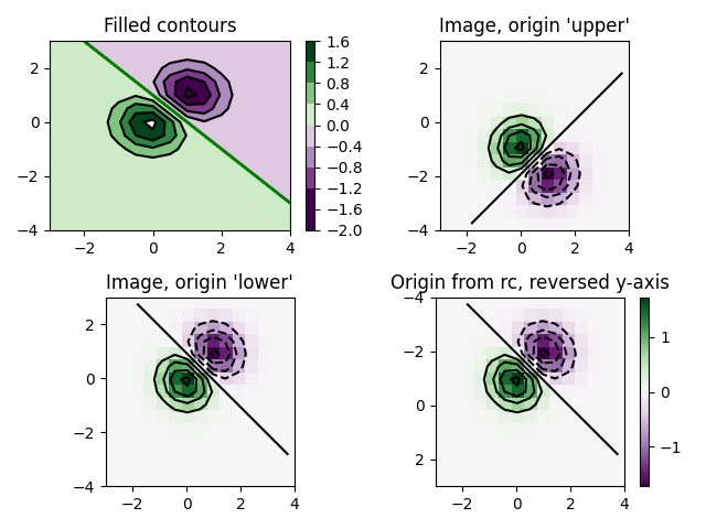
윤곽선 이미지 #

컨투어링, 채워진 컨투어링 및 이미지 플로팅의 조합을 테스트합니다. 등고선 라벨링에 대해서는 등고선 데모 예 를 참조하십시오 .

이 데모의 강조점은 윤곽선을 이미지에 올바르게 등록하는 방법과 원하는 방향으로 둘 다 지정하는 방법을 보여주는 것입니다. 특히 imshow 및 contour 에 대한 "origin" 및 "extent" 키워드 인수의 사용법에 유의하십시오.

import matplotlib.pyplot as plt
import numpy as np
from matplotlib import cm

# Default delta is large because that makes it fast, and it illustrates
# the correct registration between image and contours.
delta = 0.5

extent = (-3, 4, -4, 3)

x = np.arange(-3.0, 4.001, delta)
y = np.arange(-4.0, 3.001, delta)
X, Y = np.meshgrid(x, y)
Z1 = np.exp(-X**2 - Y**2)
Z2 = np.exp(-(X - 1)**2 - (Y - 1)**2)
Z = (Z1 - Z2) * 2

# Boost the upper limit to avoid truncation errors.
levels = np.arange(-2.0, 1.601, 0.4)

norm = cm.colors.Normalize(vmax=abs(Z).max(), vmin=-abs(Z).max())
cmap = cm.PRGn

fig, _axs = plt.subplots(nrows=2, ncols=2)
fig.subplots_adjust(hspace=0.3)
axs = _axs.flatten()

cset1 = axs[0].contourf(X, Y, Z, levels, norm=norm,
                        cmap=cmap.resampled(len(levels) - 1))
# It is not necessary, but for the colormap, we need only the
# number of levels minus 1.  To avoid discretization error, use
# either this number or a large number such as the default (256).

# If we want lines as well as filled regions, we need to call
# contour separately; don't try to change the edgecolor or edgewidth
# of the polygons in the collections returned by contourf.
# Use levels output from previous call to guarantee they are the same.

cset2 = axs[0].contour(X, Y, Z, cset1.levels, colors='k')

# We don't really need dashed contour lines to indicate negative
# regions, so let's turn them off.

for c in cset2.collections:
    c.set_linestyle('solid')

# It is easier here to make a separate call to contour than
# to set up an array of colors and linewidths.
# We are making a thick green line as a zero contour.
# Specify the zero level as a tuple with only 0 in it.

cset3 = axs[0].contour(X, Y, Z, (0,), colors='g', linewidths=2)
axs[0].set_title('Filled contours')
fig.colorbar(cset1, ax=axs[0])


axs[1].imshow(Z, extent=extent, cmap=cmap, norm=norm)
axs[1].contour(Z, levels, colors='k', origin='upper', extent=extent)
axs[1].set_title("Image, origin 'upper'")

axs[2].imshow(Z, origin='lower', extent=extent, cmap=cmap, norm=norm)
axs[2].contour(Z, levels, colors='k', origin='lower', extent=extent)
axs[2].set_title("Image, origin 'lower'")

# We will use the interpolation "nearest" here to show the actual
# image pixels.
# Note that the contour lines don't extend to the edge of the box.
# This is intentional. The Z values are defined at the center of each
# image pixel (each color block on the following subplot), so the
# domain that is contoured does not extend beyond these pixel centers.
im = axs[3].imshow(Z, interpolation='nearest', extent=extent,
                   cmap=cmap, norm=norm)
axs[3].contour(Z, levels, colors='k', origin='image', extent=extent)
ylim = axs[3].get_ylim()
axs[3].set_ylim(ylim[::-1])
axs[3].set_title("Origin from rc, reversed y-axis")
fig.colorbar(im, ax=axs[3])

fig.tight_layout()
plt.show()

채워진 윤곽선, 이미지, 원점 'upper', 이미지, 원점 'lower', rc에서 원점, 역방향 y축

참조

다음 함수, 메서드, 클래스 및 모듈의 사용이 이 예제에 표시됩니다.

Sphinx-Gallery에서 생성한 갤러리