히스토그램이 있는 산점도 #

플롯의 측면에 히스토그램으로 산점도의 주변 분포를 표시합니다.

주요 축을 주변과 잘 정렬하기 위해 두 가지 옵션이 아래에 표시됩니다.

조금 더 복잡할 수 있지만 Axes.inset_axes고정 종횡비로 기본 축을 올바르게 처리할 수 있습니다.

axes_grid1 도구 키트 를 사용하여 유사한 그림을 생성하는 대체 방법 은 Scatter Histogram(Locatable Axes) 예제에 나와 있습니다. Figure.add_axes마지막으로 (여기에 표시되지 않음) 을 사용하여 모든 축을 절대 좌표로 배치할 수도 있습니다 .

먼저 x 및 y 데이터를 입력으로 사용하는 함수를 정의하고 세 개의 축, 분산의 기본 축 및 두 개의 주변 축을 정의해 보겠습니다. 그런 다음 제공된 축 내부에 분산 및 히스토그램을 생성합니다.

import numpy as np
import matplotlib.pyplot as plt

# Fixing random state for reproducibility
np.random.seed(19680801)

# some random data
x = np.random.randn(1000)
y = np.random.randn(1000)


def scatter_hist(x, y, ax, ax_histx, ax_histy):
    # no labels
    ax_histx.tick_params(axis="x", labelbottom=False)
    ax_histy.tick_params(axis="y", labelleft=False)

    # the scatter plot:
    ax.scatter(x, y)

    # now determine nice limits by hand:
    binwidth = 0.25
    xymax = max(np.max(np.abs(x)), np.max(np.abs(y)))
    lim = (int(xymax/binwidth) + 1) * binwidth

    bins = np.arange(-lim, lim + binwidth, binwidth)
    ax_histx.hist(x, bins=bins)
    ax_histy.hist(y, bins=bins, orientation='horizontal')

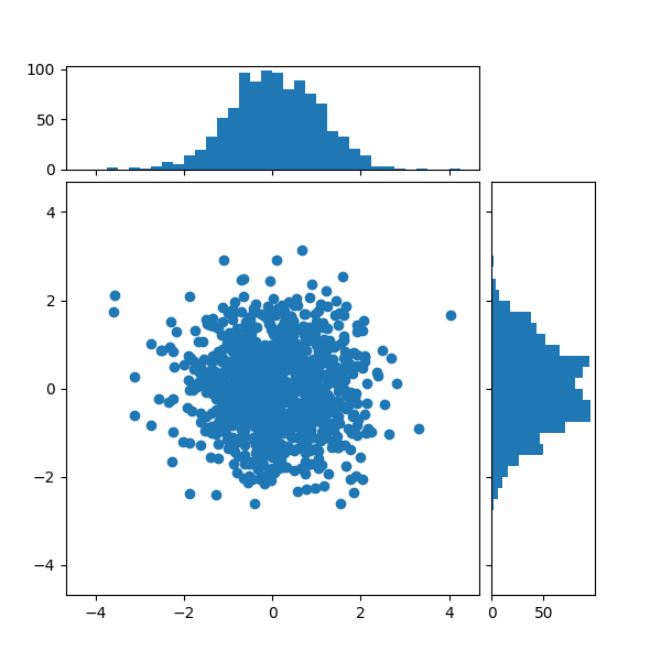
gridspec을 사용하여 축 위치 정의 #

원하는 레이아웃을 얻기 위해 폭과 높이 비율이 같지 않은 그리드 사양을 정의합니다. Figure 자습서 에서 여러 축 정렬 도 참조하십시오 .

# Start with a square Figure.
fig = plt.figure(figsize=(6, 6))
# Add a gridspec with two rows and two columns and a ratio of 1 to 4 between
# the size of the marginal axes and the main axes in both directions.
# Also adjust the subplot parameters for a square plot.
gs = fig.add_gridspec(2, 2,  width_ratios=(4, 1), height_ratios=(1, 4),
                      left=0.1, right=0.9, bottom=0.1, top=0.9,
                      wspace=0.05, hspace=0.05)
# Create the Axes.
ax = fig.add_subplot(gs[1, 0])
ax_histx = fig.add_subplot(gs[0, 0], sharex=ax)
ax_histy = fig.add_subplot(gs[1, 1], sharey=ax)
# Draw the scatter plot and marginals.
scatter_hist(x, y, ax, ax_histx, ax_histy)

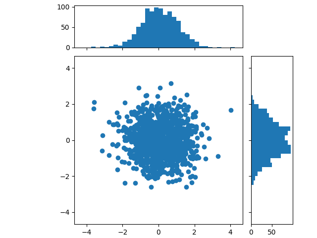
inset_axes를 사용하여 축 위치 정의하기 #

inset_axes주 축 외부 에 마진을 배치하는 데 사용할 수 있습니다 . 이렇게 하면 주요 축의 가로세로 비율을 고정할 수 있고 여백이 항상 축의 위치를 기준으로 그려질 수 있다는 장점이 있습니다.

# Create a Figure, which doesn't have to be square.
fig = plt.figure(constrained_layout=True)
# Create the main axes, leaving 25% of the figure space at the top and on the
# right to position marginals.
ax = fig.add_gridspec(top=0.75, right=0.75).subplots()
# The main axes' aspect can be fixed.
ax.set(aspect=1)
# Create marginal axes, which have 25% of the size of the main axes.  Note that
# the inset axes are positioned *outside* (on the right and the top) of the
# main axes, by specifying axes coordinates greater than 1.  Axes coordinates
# less than 0 would likewise specify positions on the left and the bottom of
# the main axes.
ax_histx = ax.inset_axes([0, 1.05, 1, 0.25], sharex=ax)
ax_histy = ax.inset_axes([1.05, 0, 0.25, 1], sharey=ax)
# Draw the scatter plot and marginals.
scatter_hist(x, y, ax, ax_histx, ax_histy)

plt.show()

참조

다음 함수, 메서드, 클래스 및 모듈의 사용이 이 예제에 표시됩니다.

스크립트의 총 실행 시간: (0분 1.217초)

Sphinx-Gallery에서 생성한 갤러리